이것이 얼마 만에 보는 수학인가..
데이터 분석을 위해 잊었던 통계지식들을 다시금 머리에 집어넣고 있는데, 한국어로도 간만인걸 영어로도 알아야하다보니
깔끔하게 정리해두는게 좋을 것 같아 해보았습니다.

참고로!
이번 포스팅에서는 순수 기술통계와 시각적인 이해, EDA 기초에 대해서만 다루었습니다:)
1. Basic Statistical Concepts (기초 통계 개념)
1.1 Key Terms (주요 용어)
Variable (변량)
- Definition: Numerical values or data points in a dataset
- Korean: 자료의 수치, 데이터의 값
- Example: Heights of 100 people randomly selected
Frequency (도수)
- Definition: Number of observations that fall within each class interval
- Korean: 각 계급에 속하는 변량의 개수
Relative Frequency (상대도수)
- Definition: Proportion of observations in each class interval
- Korean: 각 계급에 속하는 변량의 비율
- Formula: Relative Frequency = Frequency / Total Number of Observations
Class Interval (계급)
- Definition: A range of values that divides the data into groups
- Korean: 변량을 일정한 간격으로 나눈 구간
- Note: Consider minimum and maximum values when setting intervals
1.2 Types of Data (자료의 종류)
Categorical Data (범주형 자료)
- Nominal Data (명목형): Categories with no order (성별, 혈액형)
- Ordinal Data (순서형): Categories with meaningful order (학점, 만족도)
Quantitative Data (양적 자료)
- Discrete Data (이산형): Countable values (자녀 수, 판매량)
- Continuous Data (연속형): Measurable values (키, 체중, 시간)
- Interval Data (구간형): Equal intervals, no true zero (온도)
- Ratio Data (비율형): Equal intervals with true zero (소득, 나이)
2. Measures of Central Tendency (중심경향성)
Central Tendency: The tendency of data to cluster around a central value
Korean: 데이터 분포의 중심을 보여주는 값이미지 출처: "Understanding Measures of Central Tendency", Nitesh (@nitesh.py), Medium
2.1 Mode (최빈값)
- Definition: Most frequently occurring value in a dataset
- Korean: 가장 빈번하게 나타나는 값
- Best for: Categorical data (범주형 자료)
- Advantage: Can be used for any type of data
- Limitation: May not exist or may have multiple modes
2.2 Median (중앙값)
- Definition: Middle value when data is arranged in ascending order
- Korean: 자료를 크기 순으로 나열했을 때 가운데 위치하는 값
- Calculation:
- Odd n: Middle value
- Even n: Average of two middle values
- Advantage: Robust to outliers (이상치에 크게 영향받지 않음)
- Best for: Ordinal data and skewed distributions (순서형 자료, 치우친 분포)
2.3 Mean (평균)
- Definition: Sum of all values divided by number of observations
- Korean: 자료의 값을 모두 더해서 자료의 수로 나눈 값
- Formula: x̄ = Σxi / n
- Best for: Continuous data with normal distribution (연속형 자료, 정규분포)
- Disadvantage: Sensitive to outliers (이상치에 영향을 크게 받음)
2.4 Other Types of Means
Weighted Mean (가중평균)
- Definition: Average that assigns different weights to different values
- Korean: 자료의 중요도에 따라 가중치를 부여한 평균
- Formula: x̄w = Σ(wi × xi) / Σwi
- Example: GPA calculation with credit hours
Geometric Mean (기하평균)
- Definition: Average useful for rates of growth or ratios
- Korean: 성장률 등 이전 시점에 대한 비율의 평균
- Formula: GM = ⁿ√(x₁ × x₂ × ... × xₙ)
- Examples: CAGR (Compound Annual Growth Rate), investment returns
Harmonic Mean (조화평균)
- Definition: Reciprocal of arithmetic mean of reciprocals
- Formula: HM = n / Σ(1/xi)
- Use: Averaging rates (속도, 비율의 평균)
3. Measures of Dispersion (퍼짐정도)
Dispersion: How spread out the data points are from the center
Korean: 자료가 얼마나 흩어져있고 얼마나 모여있는지
3.1 Range (범위)
- Definition: Difference between maximum and minimum values
- Korean: 최대값 - 최소값
- Formula: Range = Max - Min
- Advantages: Easy to calculate and interpret
- Disadvantages:
- No information about distribution within range
- Heavily influenced by outliers (극단치에 매우 민감)
3.2 Interquartile Range (IQR)
- Definition: Q3 - Q1 (3rd quartile minus 1st quartile)
- Korean: 제3사분위수 - 제1사분위수
- Use: Better measure for skewed distributions (치우친 분포)
- Advantage: Resistant to outliers
- Application: Used in box plots for outlier detection
3.3 Variance (분산)
- Definition: Average of squared deviations from the mean
- Korean: 편차 제곱의 평균
- Formula: σ² = Σ(xi - μ)² / n (population)
- Formula: s² = Σ(xi - x̄)² / (n-1) (sample)
- Purpose: Measures variability around the mean
- Unit: Squared units of original data
3.4 Standard Deviation (표준편차)
- Definition: Square root of variance
- Korean: 분산의 제곱근
- Formula: σ = √variance
- Advantages:
- Same units as original data
- Easier to interpret than variance
- Good for standardizing data scales
4. Distribution Shape (분포의 형태)
4.1 Skewness (왜도)
- Definition: Measure of asymmetry in distribution
- Korean: 분포의 좌우 비대칭성 정도
Types of Skewness:
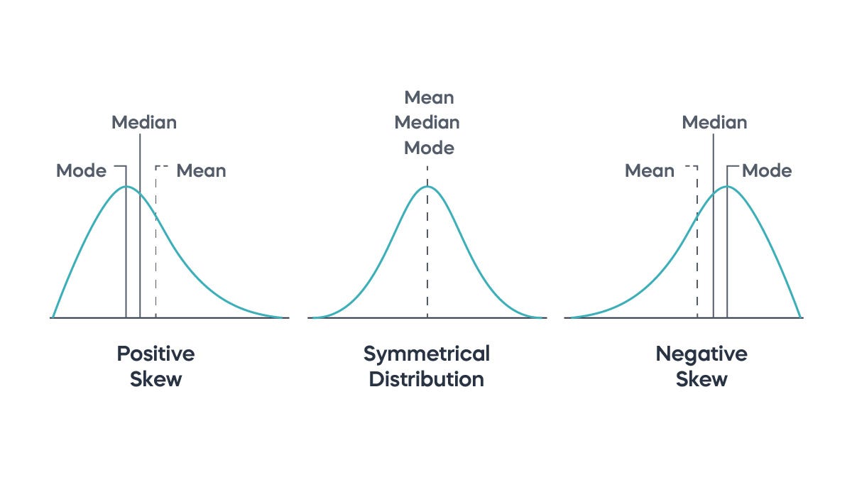
- Positive Skew (Right Skew):
- Longer right tail (오른쪽 꼬리가 긴 분포)
- Mode < Median < Mean
- 데이터 분포: 대부분의 값이 왼쪽(낮은 값)에 몰려있고, 소수의 큰 값들이 오른쪽에 있음
- Examples: 소득 분포, 집값 분포
- Zero Skew:
- Symmetric distribution (대칭 분포)
- Mean = Median = Mode
- Negative Skew (Left Skew):
- Longer left tail (왼쪽 꼬리가 긴 분포)
- Mean < Median < Mode
- 데이터 분포: 대부분의 값이 오른쪽(높은 값)에 몰려있고, 소수의 작은 값들이 왼쪽에 있음
- Examples: 연령별 사망률, 쉬운시험점수, 고품질 제품의 수명
왜도(Skewness) 치우침 판단 기준값
일반적인 기준
- -0.5 ~ +0.5: 거의 대칭적 (대부분 정규분포로 간주 가능)
- -1 ~ -0.5 또는 +0.5 ~ +1: 보통 정도의 치우침
- -1 미만 또는 +1 초과: 심하게 치우침
엄격한 기준 (일부 연구에서 사용)
- 절댓값 2 초과: 매우 심한 치우침
- 절댓값 3 초과: 극심한 치우침 (정규성 가정 심각하게 위반)
가장 보편적으로 사용되는 기준은 ±0.5와 ±1입니다.
4.2 Kurtosis (첨도)
- Definition: Measure of tail thickness and peak sharpness
- Korean: 분포의 뾰족한 정도, 양쪽 꼬리의 두터움 정도
Types of Kurtosis:
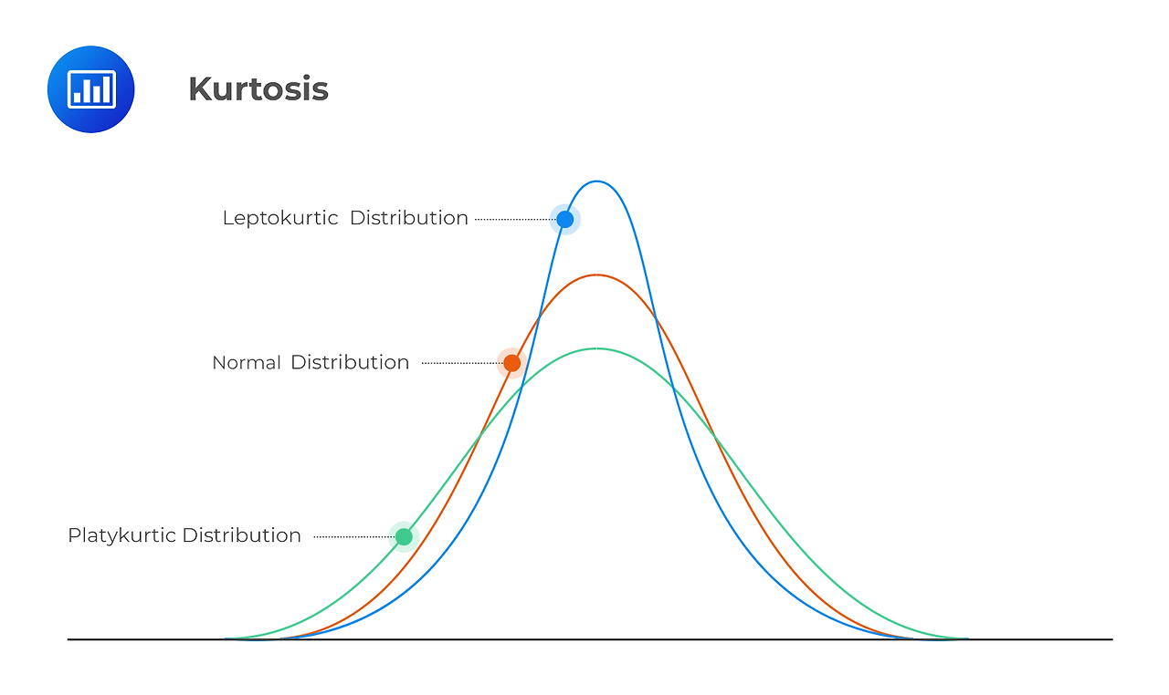
- Leptokurtic (Excess Kurtosis > 0):
- Sharp peak, thick tails (뾰족하고 두터운 꼬리)
- More extreme values than normal distribution
- Platykurtic (Excess Kurtosis < 0):
- Flat peak, thin tails (평평하고 얇은 꼬리)
- Fewer extreme values than normal distribution
- Mesokurtic (Excess Kurtosis = 0):
- Normal distribution shape (정규분포와 같은 첨도)
Important Note: High kurtosis indicates higher probability of extreme events (이상치 발생 가능성이 높음)
5. Descriptive Statistics Applications (기술통계 응용)
5.1 What is Descriptive Statistics? (기술통계란?)
- Definition: Methods to summarize and describe data characteristics
- Korean: 데이터의 간결한 요약 정보
- Purpose: Understand data patterns without making inferences
- Components: Numerical summaries + Visualizations
5.2 Descriptive vs Inferential Statistics
Aspect Descriptive Statistics Inferential Statistics
| Aspect | Descriptive Statistics | Inferential Statistics |
| Purpose | Describe sample data | Make inferences about population |
| Korean | 기술통계 | 추론통계 |
| Scope | What we observe | What we can conclude |
| Methods | Summaries, charts | Hypothesis tests, confidence intervals |
| Examples | Mean height = 170cm | Population mean likely between 165-175cm |
5.3 Five-Number Summary (다섯 수치 요약)
- Minimum (최솟값)
- Q1 (1st Quartile, 제1사분위수): 25th percentile
- Median (중앙값): 50th percentile
- Q3 (3rd Quartile, 제3사분위수): 75th percentile
- Maximum (최댓값)
Use: Foundation for box plots and outlier detection
5.4 Outlier Detection (이상치 탐지)
- IQR Method:
- Lower fence: Q1 - 1.5 × IQR
- Upper fence: Q3 + 1.5 × IQR
- Values beyond fences are potential outliers
- Z-score Method: |z| > 2 or 3 (depending on strictness)
6. Data Visualization & EDA (데이터 시각화와 탐색적 분석)
6.1 Frequency Distribution Visualization
Frequency Distribution Table (도수분포표)
- Purpose: Organize data by class intervals and their frequencies
- Components: Class intervals, frequency, relative frequency, cumulative frequency
- Advantages: Easy to understand distribution patterns
- Disadvantages: Loss of individual data points
Histogram (히스토그램)
- Definition: Visual representation of frequency distribution
- Korean: 도수분포표를 시각화하는 가장 기본적인 방법
- Features: Bars touch each other (연속된 막대)
- Use: Shows distribution shape, central tendency, spread
6.2 Other Important Visualizations
Box Plot (상자그림)
- Components: Box (IQR), whiskers, median line, outliers
- Advantages: Shows five-number summary and outliers clearly
- Use: Comparing distributions across groups
Dot Plot (점도표)
- Use: Small datasets, shows exact values
- Advantage: No loss of information
Stem-and-Leaf Plot (줄기잎그림)
- Advantage: Retains original data values
- Use: Quick visualization for small to medium datasets
6.3 Exploratory Data Analysis (EDA)
- Definition: Process of analyzing data to summarize main characteristics
- Korean: 탐색적 자료 분석
- Goals:
- Understand data structure
- Detect outliers and errors
- Find patterns and relationships
- Test assumptions
- Suggest hypotheses
EDA Steps:
- Data Quality Check: Missing values, duplicates, errors
- Univariate Analysis: Individual variable distributions
- Bivariate Analysis: Relationships between pairs of variables
- Multivariate Analysis: Relationships among multiple variables
Key Formulas Summary (주요 공식 정리)
| Statistic | Population Formula | Sample Formula | Purpose |
| Mean | μ = Σxi / N | x̄ = Σxi / n | Central tendency |
| Variance | σ² = Σ(xi - μ)² / N | s² = Σ(xi - x̄)² / (n-1) | Dispersion |
| Std Dev | σ = √σ² | s = √s² | Dispersion (same units) |
| Range | Max - Min | Max - Min | Simple spread measure |
| IQR | Q3 - Q1 | Q3 - Q1 | Robust spread measure |
Practical Guidelines for Data Analysis
When to Use Which Measure?
Central Tendency:
- Normal Distribution: Use mean
- Skewed Distribution: Use median
- Categorical Data: Use mode
- Multiple Modes: Report all modes
Dispersion:
- Normal Distribution: Use standard deviation
- Skewed Distribution: Use IQR
- Quick Overview: Use range (but report its limitations)
Distribution Shape:
- Always check skewness and kurtosis before choosing analysis methods
- Visualize first: Use histograms and box plots
- Consider transformation for highly skewed data
Data Quality Checklist:
- ✅ Check for missing values
- ✅ Identify and handle outliers
- ✅ Verify data types are correct
- ✅ Look for impossible values
- ✅ Check for duplicate records
- ✅ Validate ranges and constraints
'Study > Data Analysis' 카테고리의 다른 글
| Box Plot(상자 수염) 해석하는 법 (1) | 2025.06.16 |
|---|---|
| MySQL 기초 - 1편: DDL로 테이블 구조 마스터하기 🏗️ (1) | 2025.06.16 |
| 문과생의 통계학 기초 개념 정리 ❸ (Statistics Fundamentals for Quant Research) (2) | 2025.06.08 |
| 문과생의 통계학 기초 개념 정리 ❷ (Statistics Fundamentals for Quant Research) (2) | 2025.06.07 |
| Mac M2 MySQL 설치 (HomeBrew 설치, zsh : command not found 해결) (0) | 2025.06.06 |


